Experimental Results
Experiment Results[edit | edit source]
Analyzer[edit | edit source]
Decoding the Data[edit | edit source]
The data in the experiment came into CODA in hexadecimal form. Also, the data had a header word and two counters before the actual data. The manual had to be referenced to understand how the data was presented and how it worked. Then, the decoder had to be altered in order to properly convert the data and make it readable for the program. The main thing that had to be changed was the bitwise AND lines within the analyzer program. This made sure the data was moved over and read properly. The bitwise AND functions had to be changed to fit the specifications of the of our configuration.
TDC[edit | edit source]
Raw TDC Data[edit | edit source]
Numerous trials were run using only the TDC in order to properly configure it. Most of these trials were attempts to fix the timing and trigger so that the TDC would work properly with CODA. A macro was written to see the raw data stored in the TDC on all four of the channels. The four channels filled with raw data is displayed below.

Corrected TDC Data[edit | edit source]
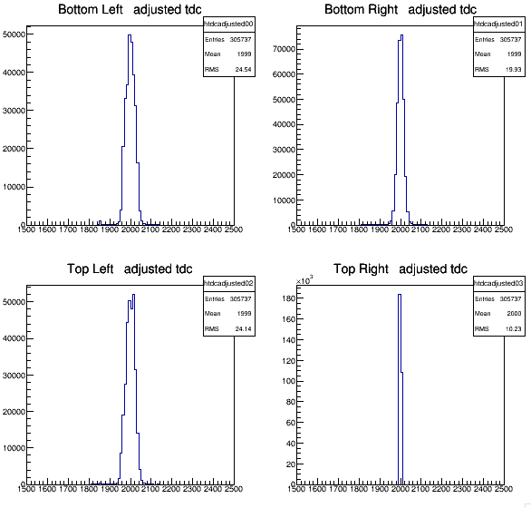
Then the data on all four channels had to be centered around a central point, in this case 2000, in order to get the other graphs to be uniform and correct. The corrected TDC data is shown here.
ADC[edit | edit source]
New Configuration[edit | edit source]
In order to run CODA properly, a new configuration had to be created. This configuration had to redirect files to the c792_775 folder where the ADC and TDC libraries and headers were held. All of the changes were simply made to the TDC configuration that was already in place. Overall, only a few minor but important changes had to be made.
Raw ADC Data[edit | edit source]
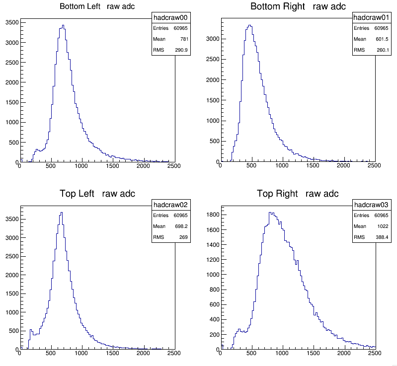
The ADC was then placed into the crate and setup properly with CODA. All of the ADC data in all four channels were placed into a graph in the same manner that the TDC was done. The raw data graphs are shown below.
Corrected TDC Data[edit | edit source]
The ADC data was then corrected just as the TDC data was. The data was centered around the 1000 point range. This corrected data graph is shown below.

Finding Energy Deposition versus Position[edit | edit source]
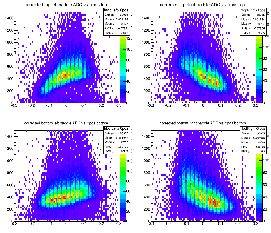
The next step was to make a two dimensional histogram of ADC data versus the position where the cosmic ray hit the scintillator. This graph was done for each of the four photomultiplier tubes. One for the top right, top left, bottom right, and bottom left. These graphs are displayed below.
Finding Theta[edit | edit source]
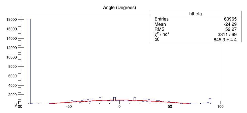
After this, the top right and top left ADC means were added together and then divided by two. This addition made the data based on two scintillators instead of the four photomultiplier tubes. Then, the angle was found in the experiment using the TDC data. An angle distribution of cosine squared was found. More angles seemed to hit toward the middle around the degree 0 than towards the edges. A graph is shown below.
Energy Deposition versus Theta[edit | edit source]
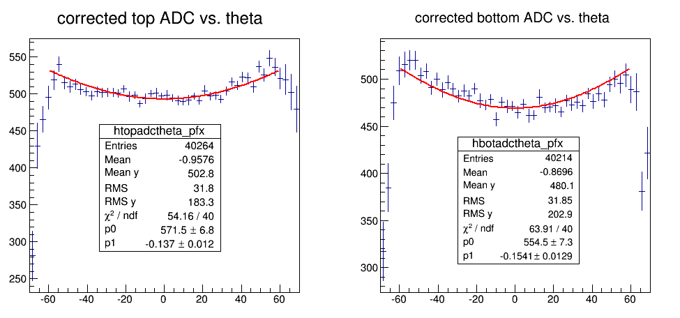
The final thing that was done was a two dimensional histogram was made comparing the top ADC versus theta. And a histogram was made comparing the bottom ADC versus theta. The graph is displayed below.

Fitting the Data[edit | edit source]
Then, a line of best fit was drawn overtop of the histogram using a object called profile in the analyzer in root. It was seen that the line of best fit needed to be a cosine curve. A graph of this line of best fit is shown below for the top and bottom scintillators.
