ROOT Analysis: Difference between revisions
en>Jlabdaq |
m 1 revision imported |
(No difference)
| |
Latest revision as of 17:59, 24 December 2024
Data Editing
Remove Extraneous Text
After the text file is copied onto a USB drive, the data can be moved to a third computer for analysis. This is done because the first two computers are in single-user mode and could not run the programs needed to analyze the data. Initially, the file will look like this:
64 bytes from 192.168.1.2: icmp_seq=0 ttl=255 time=.576 ms
64 bytes from 192.168.1.2: icmp_seq=1 ttl=255 time=.587 ms
64 bytes from 192.168.1.2: icmp_seq=2 ttl=255 time=.591 ms
64 bytes from 192.168.1.2: icmp_seq=3 ttl=255 time=.511 ms
However, the only data that is necessary is the trial number and the round-trip time. Now, we can parse through the file and remove the extra text that is not needed. Listed below are the necessary steps:
Steps
1. Mount the USB
2. Copy the files onto the analysis computer using cp /media/USB Name/File Name . (The period is in the line of code)
3. Now remove the extra text using cat File Name | sed 's/= /g' | awk '{print $6 " " $10}'
The following should be the only data displayed:
0 .576
1 .587
2 .591
3 .511
4. A new file needs to be created with this new formatting, use: cat File Name | sed 's/= /g' | awk '{print $6 " " $10}' > New File Name
5. To check if the file saved properly use: cat New File Name
6. Now we will use the "emacs" editor to clear up any extraneous text. Type emacs New File Name'
7. Use this editor to remove extra text at the bottom and top of the file, then save
8. The file is now ready for data analysis
Programming to Make a Histogram
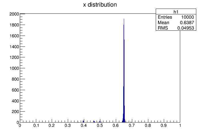
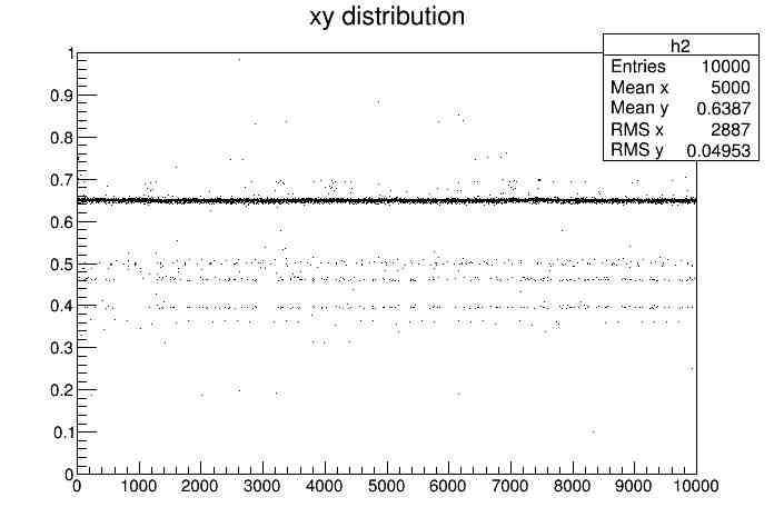
A macro was written using ROOT to store these numbers in variables and plot two histograms. The first histogram had an x-axis composed of round-trip times and the y-axis was the number of times the signal hit a certain time as shown here.
Graphing Data
Initial Graphs
This program was run in Root which is an object-oriented framework for data analysis created by CERN. Through this program, the round-trip times and trials were graphed for each of the following intervals: 1 signal per 0.0001, 0.005, 0.001, 0.05, 0.01, and 0.1 seconds. As the graph appeared, the mean, the root mean squared, and the total number of entries were also displayed.
Gauss Fit Graphs
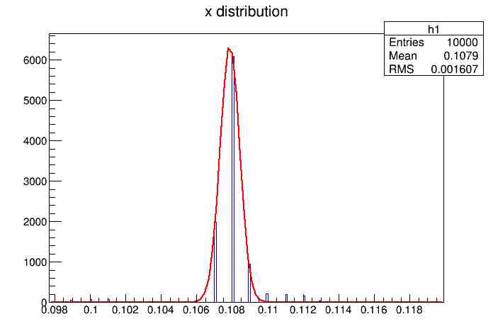
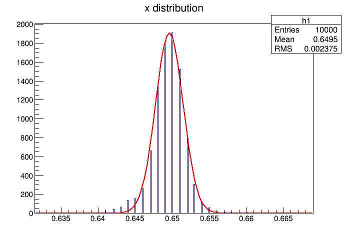
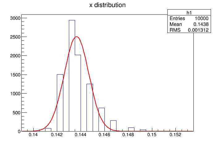
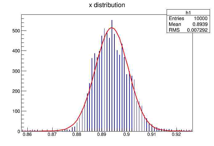
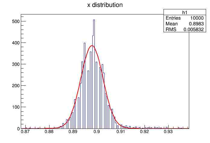
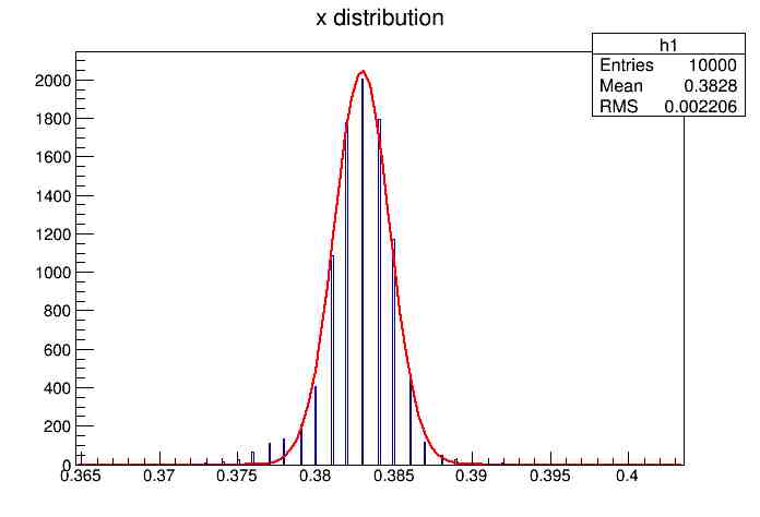
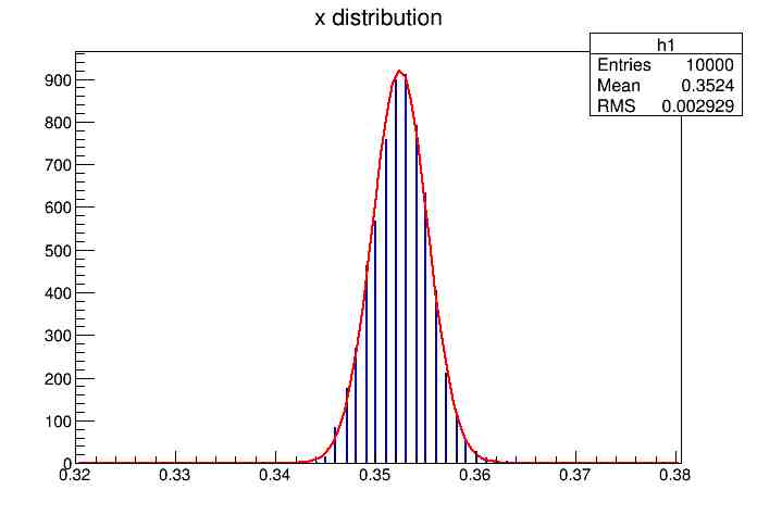
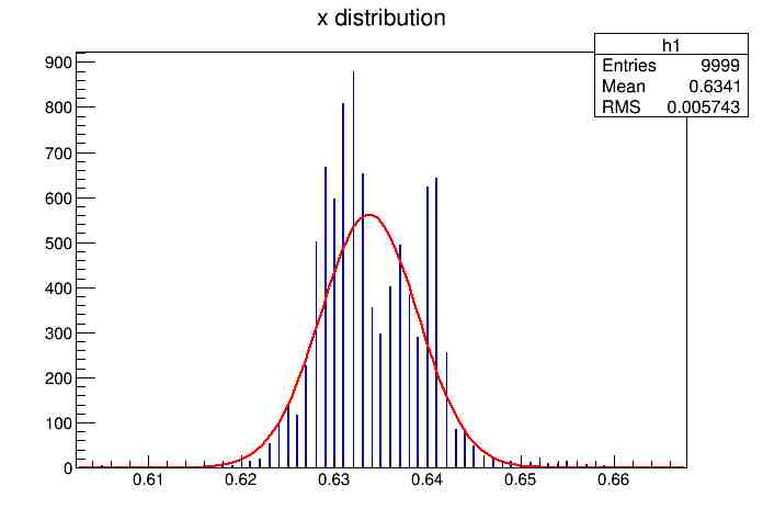
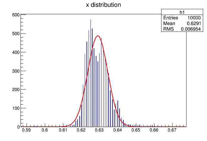
Each of these graphs was then analyzed to determine which interval had the best consistency, overall time, and accuracy. Some of these intervals resembled a normal bell curve where around 68% of the data was within one standard deviation of the mean. These intervals were then fit with a Gauss curve to see how close they actually were to being normal. This was done by another program in Root that looked at the current graph and drew a Gauss curve of best fit. Along with the curve came data defining the curve. The mean, the sigma, and the constant needed to make the curve were displayed. Here are the curves.
15.155 Meter Cable
217 Meter Cable
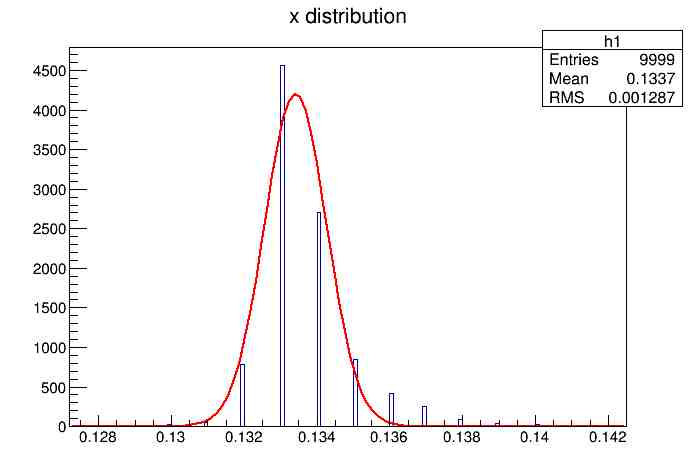
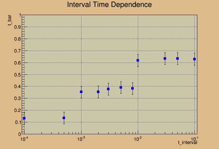
Different cable lengths needed to be used in order to see the relationship between round-trip time and cable length. It was hypothesized that a longer cable would take more time to send the same signal. This is because the signal has to travel farther and so the signal should take longer to go from one computer to the other and back. So, after the relatively short Ethernet cable was used in the first set of trials, a relatively long one was used in the second set of trials. The length of the first Ethernet cable came out to be 15.155 meters in length, and the length of the second one was 217 meters. The second set of trials are posted below.
Plotting Average Time versus Time Interval
Designing the Graph
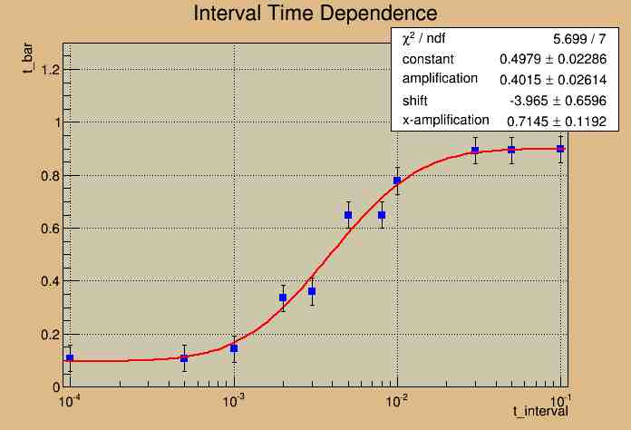
The next step was to plot the average round-trip time versus the time interval. This was done using another program in Root that accepted the mean, sigma, number of entries underneath the curve, and the root mean squared from the user. All of this data was obtained using the Gauss fit program that listed everything needed except for the number of entries underneath the curve. The total number of entries was 10000, but the total number of entries underneath the curve had to be less. So, by using the definition of the Gauss function and manipulating it, the total number of entries underneath the curve was found to be defined by sigma, the constant, a different constant, and the bin size. The equation was for the total number of entries underneath the curved was equation to y*σ*√2π*1000.
Then, the program would accept these parameters and design a logarithmic x-axis plot to display time versus interval. Also, the program was designed to put error bars were also put on the graph to show the range of means at each interval point.
Fitting the Graph
The next step was to make a fit for the graph. Since the graph had the shape of the integral of the Gauss function, the erf function was chosen to model the data. In Root, another method was created to make a line of best fit that was made to model the erf function. To better approximate the data, the erf function was scaled to the range of the data. After the best fit function was displayed the first time, the chi squared value was too high. This was mostly due to the small error bars utilized by the program. So, then, by executing many trials for the same time interval, the range of the average round-trip time interval was determined. The range of these means were approximately 0.05 seconds, so this was used as the length of the error bars. By using these error bars and the inputed data from above, the data and line of best fit was plotted on a graph as shown below.
15.155 Meter Cable
217 Meter Cable
A possible fit may be a Heaviside function or a Step Function. But more importantly, the graph illustrates that our analysis at this cable length is not the best choice for this experiment. Since our expectation of a linear fit does not match our current experimental model, changes need to be made in order to better analyze the data.
 This wiki has been closed since it has gone 30 days without activity. You may request that this wiki be reopened at