Results
Determining Ping Interval[edit | edit source]
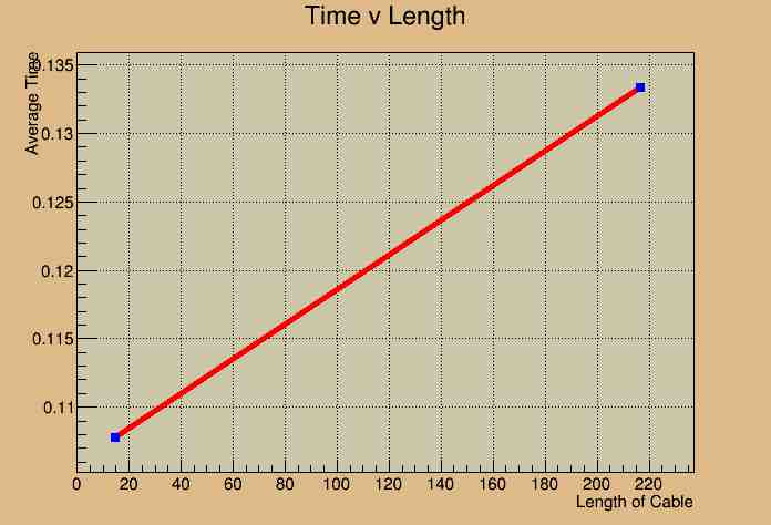
After collecting Ping data for multiple interval times using the 15 meter cable, it was determined that the 0.0001 interval time produced the most accurate results. This interval time produced the smallest ping times because there were no other background processes running. This effect is seen in the 15 meter Interval Time Dependence graph. Using 0.0001 as our interval time, we took 10 trials of 10000 pings using the 15 meter cable and 217 meter cable. The average time of the 10 trials was plotted for each cable length. The resulting graph produced a line whose slope suggested a transmission speed much faster than the speed of light.
Preparing Cable Lengths[edit | edit source]
In order to avoid any fluctuations in transmission speed in the cables, it was determined to use the same exact cable and cut it into 5 segments of varying lengths. The 217 meter cable was then cut into 1 meter, 20 meter, 40 meter, 60, meter, and 80 meter cables. The 5 resulting Cat 5 cables then had to be stripped and turned into crossover cables. In order to do this, the eight color coded wires within the cat 5 cable need to be rearranged to the crossover configuration seen in the link below and crimped within the cat 5 plug.
First Trial[edit | edit source]
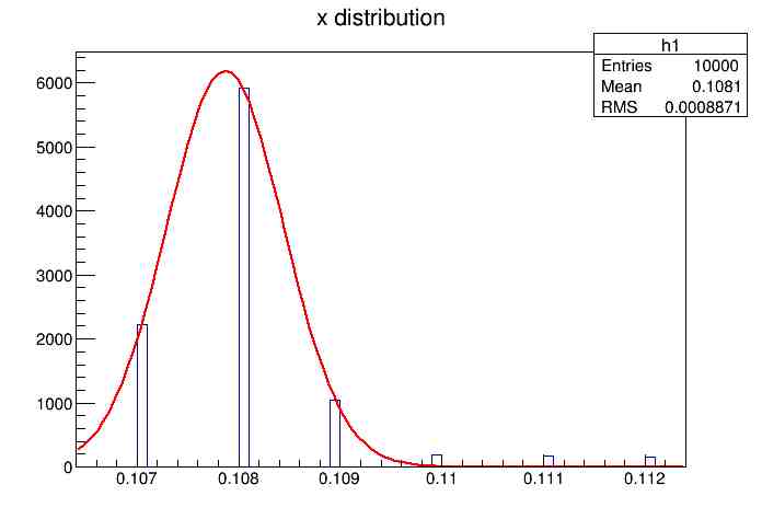
Using the 0.0001 interval time and the 5 different lengths of cable, 4 separate trials of 10000 pings were ran for each of the 5 cable lengths. A histogram for each trial was fitted using a gauss fit, and the mean from the fit of each histogram was averaged to give the mean ping time for each length of cable.
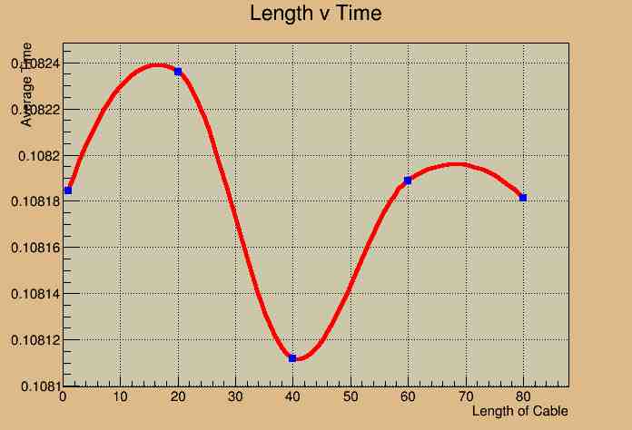
The mean times for each cable length were plotted in the graph of Cable Length versus Average Time. The resulting plot did not follow a linear fit as expected, and instead had a relation resembling a sinusoid.
It was thought that the large amount of error and inconsistency in the data might be caused by the order in which data was collected. Previously, data was collected for all four trails for a single cable length, then the cable length was changed and data collected for all four trials again. In order to reduce this statistical error, data was collected one trial at a time, while alternating between cable lengths. This would make sure that experiment was not dependent on the time between trials. With this revision in the experiment design, data was again collected and plotted in a graph of Cable Length versus Time. Error bars were added to the graph, but the results were similar to the previous experiment.
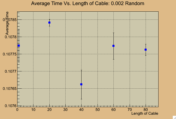
Writing Root Macro[edit | edit source]
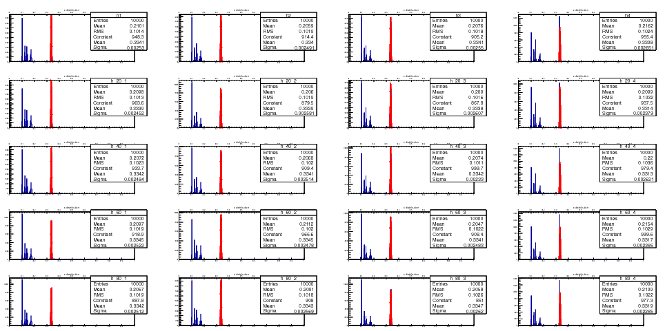
In order to simplify and streamline the analysis, a macro can be designed to read in multiple files at one time and produce several histograms of the data. Furthermore, fitting the data and illustrating the length dependence for multiple trials helps in visualizing possible errors in the data or in the analysis.
Creation[edit | edit source]
Root provides a data analysis framework that allows for program creation using a built-in C++ interpreter. Becoming familiar with Root will be key in writing functional macros that will efficiently and easily analyze our data.
Some helpful documentation has been provided by CERN to aid in learning specific functions of the framework. For instance, the following link provides an example for basic graphing syntax:
http://root.cern.ch/root/html/tutorials/graphs/graph.C.html
This type of example-based documentation may prove to be invaluable in creating Root macros.
Helpful Starting Tips[edit | edit source]
For the purposes of this experiment, histograms, graphs, fitting functions, and file I/O are going to be key for the data analysis. Below are some helpful hints on how to design such a program:
1. Have a Plan
Creating a program needs some preparation. Thinking about the end result and what you intend to produce will help greatly in designing an efficient macro. For instance, planning out possible variables, methods for parsing the data, and displaying the data can really help guide one through the creation process.
2. Scope
Along with the planning, ideas around how much data you are handling will help in deciding how to create a certain function. For example, say one experiment required five histograms to be created along with a single plot of average time versus cable length. This would be easy to simply have 5 separate Canvases with 5 different histograms and then a second Canvas to display the average time plot. But if there were 50 histograms that were going to be analyzed, a different approach would be needed for the creation of the histograms and how they are going to be displayed.
3. Attempt
Usually, a first attempt is never perfect, so do not be afraid to try something. Trial and error is going to be the best form of practice in discovering the best way to conduct the data analysis.
Useful Syntax[edit | edit source]
1. Having a Root File
Machine-Independent binary file creation: TFile *f = new TFile("junk2.root","RECREATE");
Helpful link: http://root.cern.ch/drupal/content/accessing-root-file
2. Creating Histograms
To create a single histogram pointer: TH1F *h1 = new TH1F("h1","x distribution",10000,0.0,1.0);
3. Creating Canvases
Single area mapped to a window for something to be displayed: TCanvas *c1 = new TCanvas("c1","Hists with different scales",2000,1000);
Helpful link: http://root.cern.ch/root/html/TCanvas.html
4. Pads
Dividing the canvas into columns and rows: c1->Divide(4,5);
Helpful link: http://root.cern.ch/drupal/content/canvases-and-pads
5. File I/O
String formatting might be a possible way of scanning each file: sprintf(name, "exp0_trial%d.txt",1);
Scanning file: fscanf(fp,"%f %f",&column1, &column2);
Helpful hint: TString has a function called Form() that can manipulate strings.
6. Graphing
Basic graph creation: graph = new TGraph(2,length,average_time);
Helpful link: ftp://root.cern.ch/root/doc/4Graphs.pdf
Trials After Macro[edit | edit source]
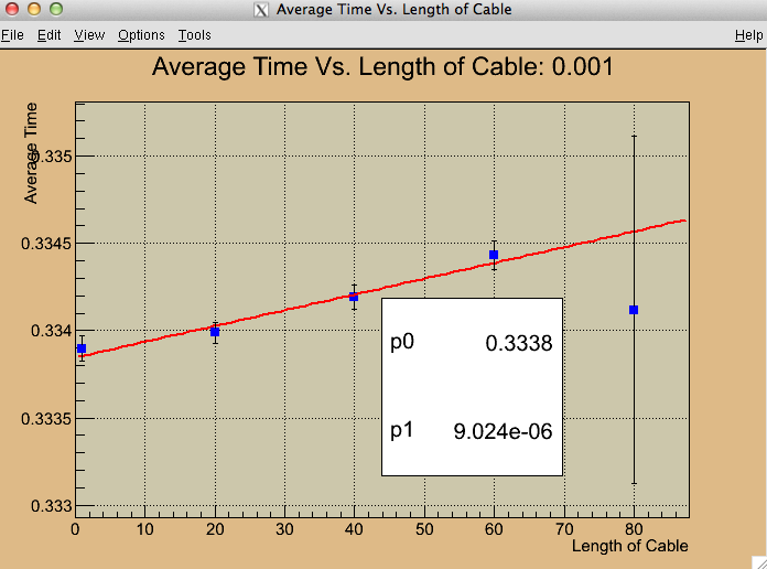
After creating a Root macro that can easily extract and graph data from 4 trials of 5 different cable lengths, more trials were ran with varying interval times. Based on the previous graphs of length versus time, it was thought that the 0.0001 interval time was too fast to produce accurate results. With that interval time, the next ping signal is sent before the previous can even finish being processed by the computer, and this creates significant systematic error in the data. To avoid this issue, data was collected in the same manner as before, but using a 0.001 interval time. The macro was plotted histograms for each trial per cable length and created a graph relating the cable length and round-trip time.

The experiment with the 0.001 interval time was repeated with similar results; the average round-trip time gradually increases as cable length increases in a linear manner. To reduce more systematic error, the order in which the cable lengths were used to collect data was randomized. When this data was plotted, the error greatly decreased and the graph was more consistent and fitted linearly.
Changing Interval Times[edit | edit source]
After evaluating the graphs of average time versus cable length for both the 0.0001 and 0.001 time intervals, trials of the same procedure were ran for 0.0015, 0.002, 0.005, and 0.0005 time intervals to try to determine the upper and lower bounds in which the data keeps consistent and a positive linear fit.
0.0015[edit | edit source]
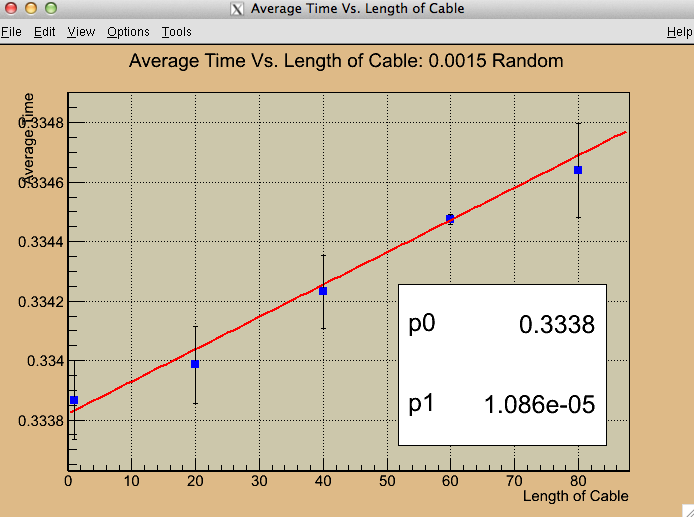
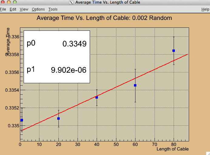
The graphs of the two closest intervals to 0.001, 0.0015 and 0.002, both produced positive linear fits with similar slopes to the 0.001 interval time.
0.002[edit | edit source]
0.005[edit | edit source]
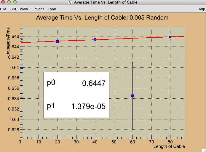
As the interval times get further away from 0.001, the graphs become more inconsistent and lose their linear fit.
0.0005[edit | edit source]
The graph of the 0.005 time interval resembles the sinusoidal graph of 0.0001 time interval.
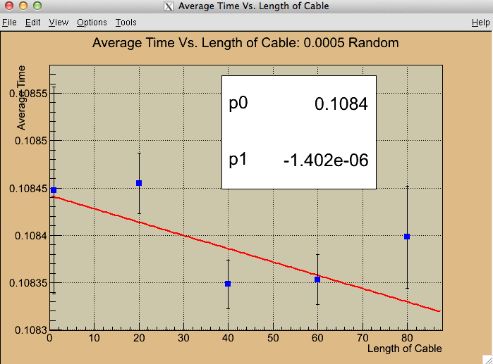
From these graphs of average time versus cable length, it was determined that the best interval time to use is 0.001.
Evaluating Slopes[edit | edit source]
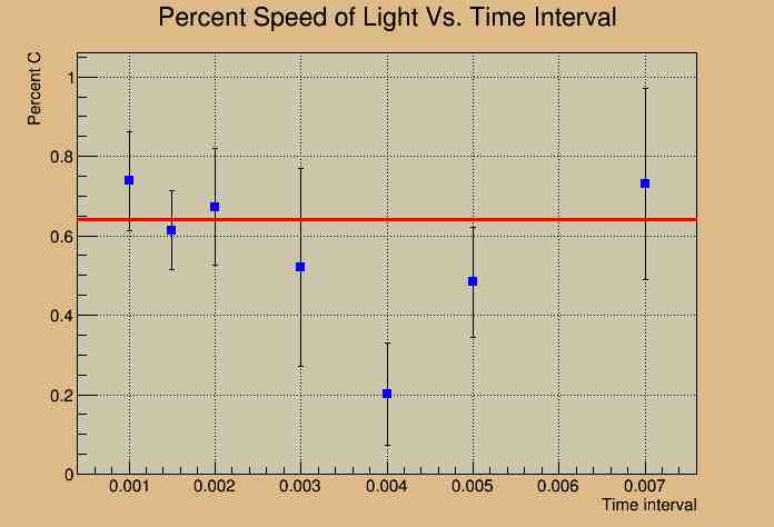
Using the graph of average time versus cable length with the 0.002 time interval, the slope of the linear fit can be used to determine the transmission speed through the wire. The axis of the graph were such that the inverse of the slope of the graph gives the transmission speed in milliseconds per meter. The x-axis is represents the length of the cable, and not the total distance travelled by the signal. To account for the signal completing a round-trip, the distances have to be multiplied by 2. After completing this, the slope of the 0.002 graph gives a transmission speed of 2.02±0.42 x 10⁸ m/s.
