Theory: Difference between revisions
en>Ryan No edit summary |
m 1 revision imported |
| (One intermediate revision by one other user not shown) | |
(No difference)
| |
Latest revision as of 17:59, 24 December 2024

The Purpose[edit | edit source]
The purpose of the Kater Pendulum experiment is to measure the local value of gravity, $ g $.
The Device[edit | edit source]
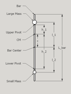
Kater’s pendulum is a physical pendulum composed of a metal rod with two knife edge pivots towards each end of the rod. The exact location of the knife edges, relative to the ends of the rod, is not of extreme importance, as long as they are relatively symmetrical. However, the distance between the knife edges must be measured precisely* enough to achieve the level of accuracy desired in the experiment. There is a weight attached to each end of the pendulum. These two masses are of different weights. This is done intentionally and is the reason Kater's Pendulum works. The pendulum can be suspended by the knife edges and set to swinging by resting either knife edge on a flat, level surface in the small mass down (SMD) and small mass up (SMU) orientations. The "large" weight is attached at a fixed position and the small weight is adjustable. This adjustment allows the pendulum's period to be adjusted. As an improvement to the pendulum design, a thin "needle" has been attached to each end of the pendulum. As the period must be measured very precisely (see Uncertainties), these "needles" allow for a smaller angle of oscillation while still allowing the pendulum to pass through a photogate.
The Theory[edit | edit source]

When displaced, the restoring force acting on the pendulum is:
- $ \tau =M_{T}gh_{1}\sin \theta $
With $ \theta $ being the angle of displacement and the pendulum orientated small mass down (SMD), $ M_{T} $ being the total mass of the system, $ g $ being local gravity, and $ h_{1} $ being the distance from the pivot to the center of mass of the system. Applying Newton's Second Law rotational analog results in:
- $ M_{T}gh_{1}\sin \theta =-{\ddot {\theta }}\mathbb {I} _{smd} $
Where $ \mathbb {I} _{smd} $ is the moment of inertia. Of course, when $ \theta $ is small, the resulting equation can be simplified to:
- $ {\ddot {\theta }}+{\frac {M_{T}gh_{1}}{\mathbb {I} _{smd}}}\theta =0 $
Solving the differential equation results in:
- $ \theta =A\cos {\left(\omega _{0}t\right)}+B\cos {\left(\omega _{0}t\right)} $
Where:
- $ \omega _{0}={\sqrt {\frac {M_{T}gh_{1}}{\mathbb {I} _{smd}}}} $
resulting in:
- $ T_{smd}=2\pi {\sqrt {\frac {\mathbb {I} _{smd}}{M_{T}gh_{1}}}} $
Where, $ T_{smd} $ is the period in the SMD orientation. Similarly, we can solve for the pendulum in the small mass up (SMU) orientation which results in:
- $ T_{smu}=2\pi {\sqrt {\frac {\mathbb {I} _{smu}}{M_{T}gh_{2}}}} $
An application of the parallel axis theorm results on the equations:
- $ \mathbb {I} _{smd}=\mathbb {I} _{cm}+M_{T}h_{1}^{2} $
and
- $ \mathbb {I} _{smu}=\mathbb {I} _{cm}+M_{T}h_{2}^{2} $
Where $ \mathbb {I} _{cm} $ is the moment of inertia about the center of mass. By substituting these equations into our previous equations for $ T $ we get:
- $ T_{smd}=2\pi {\sqrt {\frac {\mathbb {I} _{cm}+M_{T}h_{1}^{2}}{M_{T}gh_{1}}}} $
and
- $ T_{smu}=2\pi {\sqrt {\frac {\mathbb {I} _{cm}+M_{T}h_{2}^{2}}{M_{T}gh_{2}}}} $
Now, if we can find a small mass position such that our period is the same in both the SMU and SMD orientation, we can set these equations equal to one another and solving for $ \mathbb {I} _{cm} $ we find:
- $ \mathbb {I} _{cm}=M_{T}h_{1}h_{2} $
Substituting this value into either equation for period results in:
- $ T=2\pi {\sqrt {\frac {h_{1}+h_{2}}{g}}} $
And, since the distance, $ l $, between the pivots is the sum of $ h_{1} $ and $ h_{2} $ and we know this distance very well, we can write:
- $ T=2\pi {\sqrt {\frac {l}{g}}} $
or
- $ g={\frac {4\pi ^{2}l}{T^{2}}} $
With this relationship, all we need to determine $ g $ is, the period of Kater's pendulum when the small mass is adjusted such that the period when swung in the SMU orientation is identical to the period in the SMD orientation.
Some points to consider are if the weights are of different volume -which in our current pendulum, they are- their cross-sectional area will affect results due to air resistance. Also, if the weights are positioned very asymmetrically, the effect of air resistance will affect the results. The small angle approximation has been used to determine the values and the data should be corrected for this.
A Starting Estimation from First Principles[edit | edit source]

If we know the geometry and make up of the pendulum with a reasonable degree of accuracy, we are able to calculate where the small mass should be position so that it will produce the same period in the SMU and SMD orientation.
Variable Definitions[edit | edit source]
- $ M\rightarrow $ weight of large mass
- $ m\rightarrow $ weight of small mass
- $ M_{bar}\rightarrow $ weight of bar
- $ M_{T}=M+m+M_{bar}\rightarrow $ total weight
- $ L_{bar}\rightarrow $ length of bar
- $ g\rightarrow $ gravity
- $ R_{m}\rightarrow $ radius of small mass
- $ R_{M}\rightarrow $ radius of large mass
- $ \mathbb {R} \rightarrow $ radius of gyration
- $ \mathbb {I} \rightarrow $ moment of inertia
Equation of Center of Mass[edit | edit source]
- $ x={\frac {Ml_{1}-ml_{2}}{M+m+M_{bar}}} $
Equations from the Pendulum Measurements[edit | edit source]
- $ D=h_{1}+h_{2} $
- $ h_{2}-x={\frac {D}{2}} $
- $ h_{1}+x={\frac {D}{2}} $
Combining these equations results in:
- $ x={\frac {h_{2}-h_{1}}{2}} $
Equations of Period and Moment of Inertia[edit | edit source]
- $ T_{i}^{2}={\frac {4\pi ^{2}}{g}}\left({\frac {\mathbb {I} _{i}}{M_{T}h_{i}}}\right) $
- $ \mathbb {I} _{i}=M_{T}\left(\mathbb {R} ^{2}+h_{i}^{2}\right) $
- $ T_{i}^{2}={\frac {4\pi ^{2}}{g}}\left({\frac {h_{i}^{2}+\mathbb {R} ^{2}}{h_{i}}}\right) $
if $ T_{1}=T_{2} $ then:
- $ {\frac {h_{1}^{2}+\mathbb {R} ^{2}}{h_{1}}}={\frac {h_{2}^{2}+\mathbb {R} ^{2}}{h_{2}}} $
- $ h_{1}h_{2}=\mathbb {R} ^{2} $
- $ \mathbb {I} _{cm}=\mathbb {R} ^{2}\left(M_{T}\right) $
- $ \mathbb {I} _{cm}^{sys}=\mathbb {I} _{M}^{cm}+\mathbb {I} _{m}^{cm}+\mathbb {I} _{bar}^{cm} $
- $ \mathbb {I} _{M}^{cm}={\frac {1}{2}}MR_{M}^{2}+M\left(l_{1}-x\right)^{2} $
- $ \mathbb {I} _{m}^{cm}={\frac {1}{2}}mR_{m}^{2}+m\left(l_{2}+x\right)^{2} $
- $ \mathbb {I} _{M}^{bar}=\mathbb {I} _{bar}+M_{bar}x^{2} $
- $ \mathbb {I} _{bar}={\frac {1}{12}}M_{bar}L^{2} $
All of which result in:
- $ h_{1}h_{2}={\frac {1}{M+m+M_{bar}}}\left[{\frac {1}{2}}MR_{M}^{2}+M\left(l_{1}-x\right)^{2}+{\frac {1}{2}}mR_{m}^{2}+m\left(l_{2}+x\right)^{2}+{\frac {1}{12}}M_{bar}L^{2}+M_{bar}x^{2}\right] $
This is a somewhat difficult equation to solve. However, with the power and speed of modern computing, we don't have to. The following is a piece of code that finds a solution iteratively.
Iterative Solution[edit | edit source]
#include <iostream>
#include <TMath.h>
void solve() {
    // Author: Edward J. Brash
    TCanvas *c1 = new TCanvas("c1","Kater's Pendulum",800,800);
    c1->SetFillColor(42);
    c1->SetGrid();
    double x, M, m, Mbar, l1, h1, h2, D, L, rhs, lhs, Icm;
    double l2[1000],t1[1000],t2[1000];
    double g=9.810;
    double Pi=3.14159265;
    M=1.35928;
    m=0.72705;
    Mbar=2.90;
    D=0.9990;
    L=1.523;
    l1=D/2.0+0.0135+0.047523;
    double diff=1.0e99;
    double olddiff=1.0e99;
    int index=0;
    for(int i=0; i<1000; i++){
        l2[i]=0.500+(i/1000.0)*0.250;
        x=(M*l1-m*l2[i])/(M+m+Mbar);
        h2=D/2.0+x;
        h1=D/2.0-x;
        rhs=h1*h2;
        Icm=1.0/12.0*Mbar*L*L+Mbar*x*x+M*(l1-x)*(l1-x)+m*(l2[i]+x)*(l2[i]+x);
        lhs=Icm/(M+m+Mbar);
        diff = rhs-lhs;
        if (fabs(diff)<olddiff){olddiff=diff;index=i;}
        t1[i]=2*Pi*sqrt((h1*h1+lhs)/(g*h1));
        t2[i]=2*Pi*sqrt((h2*h2+lhs)/(g*h2));
        cout << l2[i] << " " << t1[i] << " " << t2[i] << endl;
        //cout << "i = "<<i<<" l2 = "<<l2[i]<<" rhs = "<<rhs<<" lhs = "<<lhs<<endl;
    }
    cout << "L2 position = " << l2[index] << " L1 position = " << l1 << endl;
    cout << "Predicted period T = " << t1[index]<< endl;
    TGraph *gra = new TGraph(1000,l2,t1);
    TGraph *grb = new TGraph(1000,l2,t2);
    gra->Draw("AP");
    grb->Draw("P");
    c1->Update();
    c1->GetFrame()->SetFillColor(21);
    c1->GetFrame()->SetBorderSize(12);
    c1->Modified();
}